Coming to the third part of the series. In this article I would be explain the concept of Deep Feedforward Networks.
Deep feedforward networks, also often called feedforward neural networks, or multilayer perceptrons(MLPs), are the quintessential deep learning models. The goal of a feedforward network is to approximate some function f*. For example, for a classifier, y = f*(x) maps an input x to a category y. A feedforward network defines a mapping y = f(x;θ) and learns the value of the parameters θ that result in the best function approximation.(Reference)
These models are called feedforward because information flows through the function being evaluated from x, through the intermediate computations used to define f, and finally to the output y. There are no feedback connections in which outputs of the model are fed back into itself. When feedforward neural networks are extended to include feedback connections, they are called recurrent neural networks(we will see in later segment).
As we know the inspiration behind neural networks are our brains. So lets see the biological aspect of neural networks.

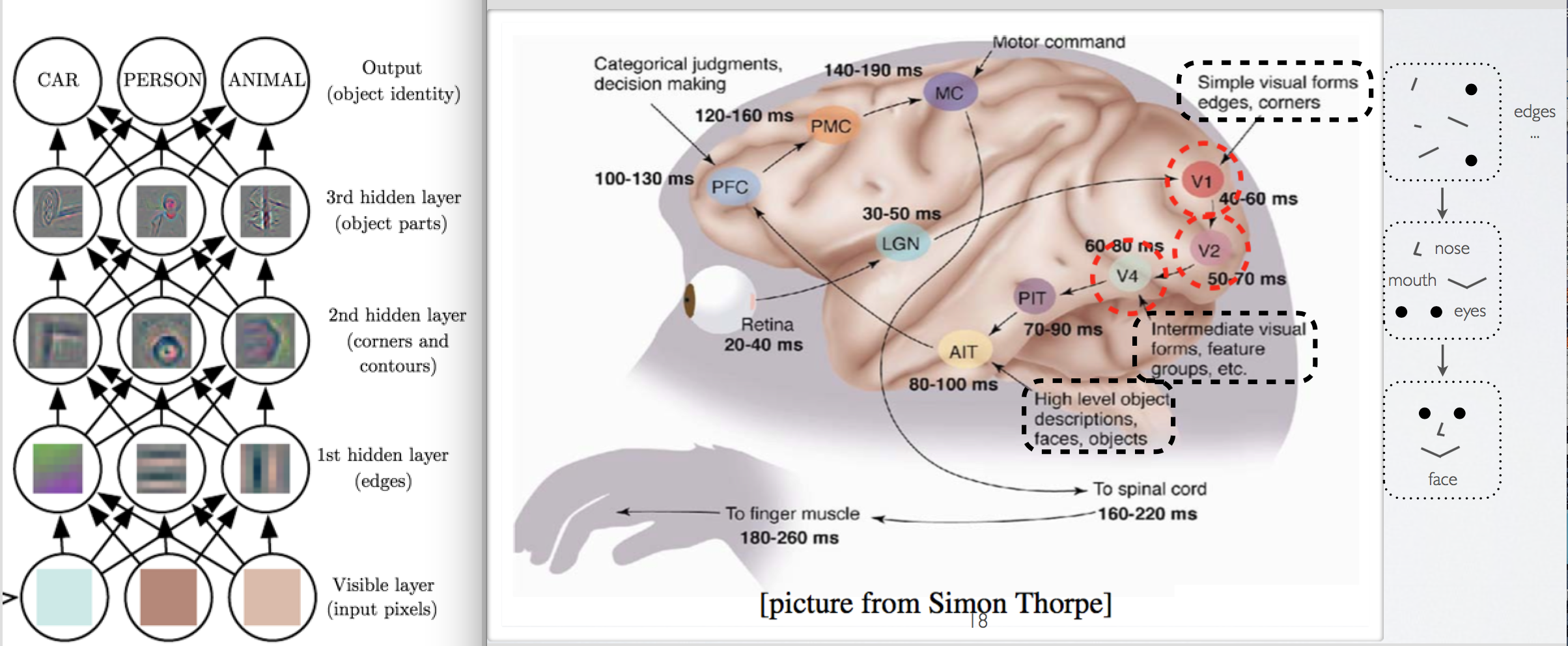
Visualising the two images in Fig 1 where the left image shows how multilayer neural network identify different object by learning different characteristic of object at each layer, for example at first hidden layer edges are detected, on second hidden layer corners and contours are identified. Similarly in our brain there are different regions for the same purpose, as we can the region denoted by V1, identifies edges, corners and etc.
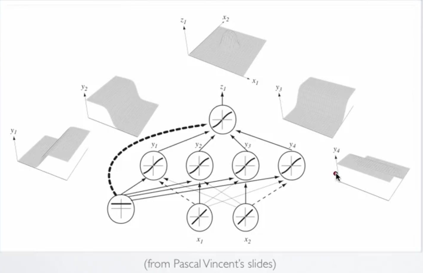
As we can see by applying neural network we can overcome the problem of non linearity(Fig 2). As we can observe in Fig 2 that neural network has trained a model by combining different distribution in one desirable distribution considering the non linearity of the problem.

Neural network emerged from a very popular machine learning algorithm named perceptron. Perceptrons were developed in the 1950s and 1960s by the scientist Frank Rosenblatt, inspired by earlier work by Warren McCulloch and Walter Pitts. As I am focusing on neural networks, please reading more about perceptron from this link(Contains a beautiful explanation of Perceptron). A famous experiment link. Combining many layer of perceptrons is known as multilayer perceptrons or feedforward neural networks.

In perceptron where neuron output value 0 and 1 based on, if the weighted sum ∑ᵢwᵢxᵢ is less than or greater than some threshold value respectively. In this post the main neuron model used in neural network architecture is one called the sigmoid neuron. In later post we will see more neuron models and their importance and applications.
Why we need new neuron model?
Suppose we have a network of perceptrons that we’d like to use to learn to solve some problem. For example, the inputs to the network might be the raw pixel data from a scanned, handwritten image of a digit. And we’d like the network to learn weights and biases so that the output from the network correctly classifies the digit. To see how learning might work, suppose we make a small change in some weight (or bias) in the network. What we’d like is for this small change in weight to cause only a small corresponding change in the output from the network. As we’ll see in a moment, this property will make learning possible. But as it occur a small change in weights leads to a big change in output. So using a neuron model like sigmoid can solve this issue. Let’s see How?

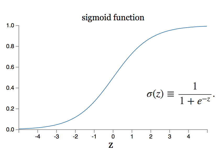
Let first see the behaviour of sigmoid function Fig 4. Unlike piecewise linear units, sigmoidal units saturate across most of their domain — they saturate to a high value when z is very positive, saturate to a low value when z is very negative, and are only strongly sensitive to their input when z is near 0. This property of sigmoid function solves our problem.
The architecture of neural networks
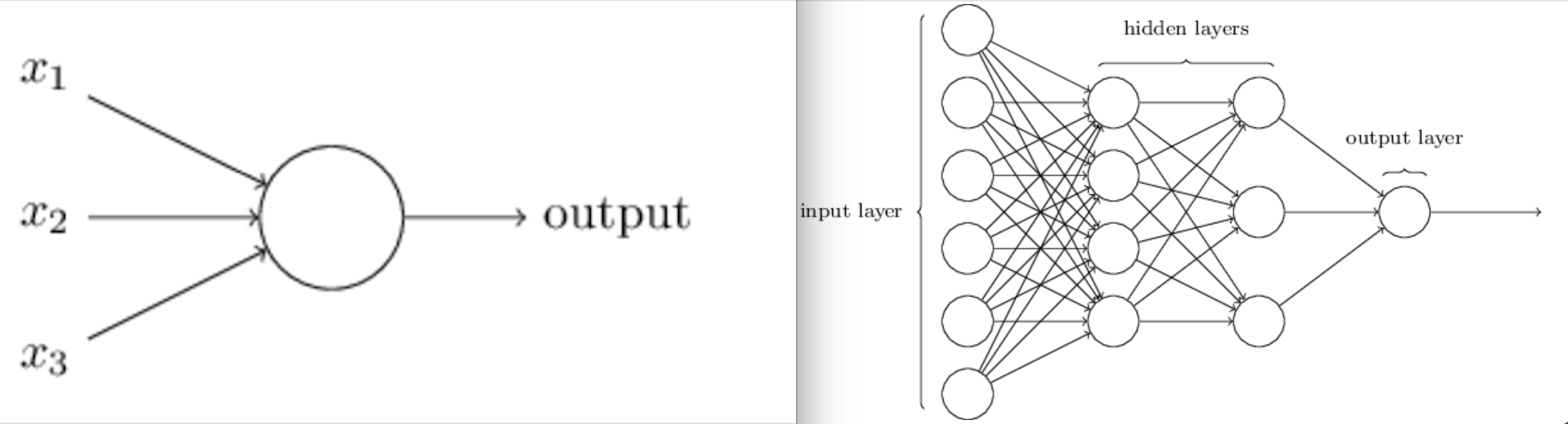
The leftmost layer in this network is called the input layer, and the neurons within the layer are called input neurons. The rightmost or output layer contains the output neurons, or, as in this case, a single output neuron. The middle layer is called a hidden layer, since the neurons in this layer are neither inputs nor outputs.

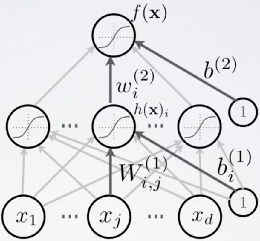
As denoted in figure wˡᵢ denote the weight of the iᵗʰ neuron of lᵗʰ layer. Wˡ₍i,j₎ denote the weight for the connection from the jᵗʰ neuron in the (l−1)ᵗʰ layer to the iᵗʰ neuron in the lᵗʰ layer. We use bᵢ for the bias for the iᵗʰ neuron. h(x) is the activation function and for now we are using sigmoid for this purpose. f(x) is output function. Refer Fig 5. Interesting thing about Feedforward networks with hidden layers is that, it provides a universal approximation framework. Specifically, the universal approximation theorem(Horniket al., 1989; Cybenko, 1989) states that a feedforward network with a linear output layer and at least one hidden layer with any “squashing” activation function (such as the sigmoid activation function) can approximate any Borel measurable function from one finite-dimensional space to another with any desired non-zero amount of error, provided that the network is given enough hidden units. The universal approximation theorem says that there exists a network large enough to achieve any degree of accuracy we desire, but the theorem does not say how large this network will be.
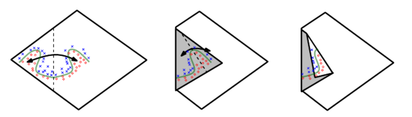
Let see how it works by taking an example. Figure 6 illustrates how a network with absolute value rectification creates mirror images of the function computed on top of some hidden unit, with respect to the input of that hidden unit. Each hidden unit specifies where to fold the input space in order to create mirror responses (on both sides of the absolute value nonlinearity). By composing these folding operations, we obtain an exponentially large number of piecewise linear regions which can capture all kinds of regular (e.g., repeating) patterns.

Cost Function
We will introduce a cost function for the purpose of solving and training our model. Now you must be thinking, Why not try to maximize that number of correct output directly, rather than minimizing a proxy measure like the quadratic cost? The problem with that is that the number of correct classified data point is not a smooth function of the weights and biases in the network. For the most part, making small changes to the weights and biases won’t cause any change at all in the number of training data point classified correctly. That makes it difficult to figure out how to change the weights and biases to get improved performance. If we instead use a smooth cost function like the quadratic cost it turns out to be easy to figure out how to make small changes in the weights and biases so as to get an improvement in the cost. That’s why we focus first on minimizing the quadratic cost, and only after that will we examine the classification accuracy. In this post we will only see mean square error cost function.


Here, w denotes the collection of all weights in the network, b all the biases, n is the total number of training inputs, a is the vector of outputs from the network when x is input, and the sum is over all training inputs, x. Of course, the output a depends on x, w and b, but to keep the notation simple I haven’t explicitly indicated this dependence. The notation ‖v‖ just denotes the usual length function for a vector v. We’ll call C the quadratic cost function; it’s also sometimes known as the mean squared error or just MSE.
Gradient-Based Learning
Designing and training a neural network is not much different from training any other machine learning model with gradient descent. The largest difference between the linear models we have seen so far and neural networks is that the nonlinearity of a neural network causes most interesting loss functions to become non-convex. This means that neural networks are usually trained by using iterative, gradient-based optimizers that merely drive the cost function to a very low value, rather than the linear equation solvers used to train linear regression models or the convex optimization algorithms with global convergence guarantees used to train logistic regression or SVMs.

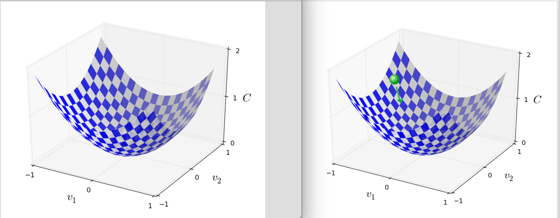
As we can see at right of figure 8, an analogy of a ball dropped in a deep valley and it settle downs at the bottom of the valley. Similarly we want our cost function to get minimize and get to the minimum value possible. When we move the ball a small amount Δv1 in the v1 direction, and a small amount Δv2 in the v2 direction. Calculus tells us that C changes as follows:


Change of the v1 and v2 such that the change in cost is negative is desirable. We can also denote ΔC≈∇C⋅Δv. where ∇C is,


and Δv is,


Indeed, there’s even a sense in which gradient descent is the optimal strategy for searching for a minimum. Let’s suppose that we’re trying to make a move Δv in position so as to decrease C as much as possible. We’ll constrain the size of the move so that ‖Δv‖=ϵ for some small fixed ϵ>0. In other words, we want a move that is a small step of a fixed size, and we’re trying to find the movement direction which decreases C as much as possible. It can be proved that the choice of Δv which minimizes ∇C⋅Δv is Δv=−η∇C, where η=ϵ/‖∇C‖ is determined by the size constraint ‖Δv‖=ϵ. So gradient descent can be viewed as a way of taking small steps in the direction which does the most to immediately decrease C. Now that the gradient vector ∇C has corresponding components ∂C/∂w𝑘 and ∂C/∂b𝓁. Writing out the gradient descent update rule in terms of components, we have


Now there are many challenges in training gradient based learning. But for now I just want to mention one problem. When the number of training inputs is very large this can take a long time, and learning thus occurs slowly. An idea called stochastic gradient descent can be used to speed up learning. To make these ideas more precise, stochastic gradient descent works by randomly picking out a small number m of randomly chosen training inputs. We’ll label those random training inputs X1,X2,…,Xm and refer to them as a mini-batch. Provided the sample size mm is large enough we expect that the average value of the ∇CXj will be roughly equal to the average over all ∇Cx, that is,


This modification helps us in reducing a good amount of computational load. Stochastic gradient descent applied to non-convex loss functions has no such convergence guarantee, and is sensitive to the values of the initial parameters. For feedforward neural networks, it is important to initialize all weights to small random values. The biases may be initialized to zero or to small positive values.We will see How can we make this calculation fast by using back propagation algorithm in next post(reference).
Thanks for reading.


